


How the Radix Sort Algorithm Works
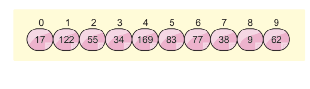
Let’s assume we have the following array list, and we want to sort this array using the radix sort:
We are going to use two more concepts in this algorithm, which are:
1. Least Significant Digit (LSD): The exponent value of a decimal number close to the rightmost position is the LSD.
For example, the decimal number “2563” has the least significant digit value of “3”.
2. Most Significant Digit (MSD): The MSD is the LSD’s exact inverse. An MSD value is the non-zero leftmost digit of any decimal number.
For example, the decimal number “2563” has the most significant digit value of “2”.
Step 1: As we already know, this algorithm works on the digits to sort the numbers. So, this algorithm requires the maximum number of digits for the iteration. Our first step is to find out the maximum number of elements in this array. After finding the maximum value of an array, we have to count the number of digits in that number for the iterations.
Then, as we have already found out, the maximum element is 169 and the number of digits is 3. So we need three iterations to sort the array.
Step 2: The least significant digit will make the first digit arrangement. The following image indicates we can see that all the smallest, least significant digits are arranged on the left side. In this case, we are focusing on the least significant digit only:
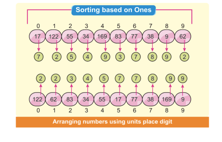
Note: Some digits are automatically sorted, even if their unit digits are different, but others are the same.
For example:
The numbers 34 at index position 3 and 38 at index position 7 have different unit digits but have the same number 3. Obviously, number 34 comes before number 38. After the first element arrangements, we can see that 34 comes before 38 automatically sorted.
Step 4: Now, we will arrange the elements of the array through the tenth place digit. As we already know, this sorting has to be finished in 3 iterations because the maximum number of elements has 3 digits. This is our second iteration, and we can assume most of the array elements will be sorted after this iteration:
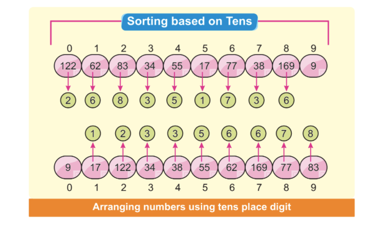
The previous results show that most array elements have already been sorted (below 100). If we had only two digits as our maximum number, only two iterations were enough to get the sorted array.
Step 5: Now, we are entering the third iteration based on the most significant digit (hundreds place). This iteration will sort the three-digit elements of the array. After this iteration, all elements of the array will be in sorted order in the following manner:
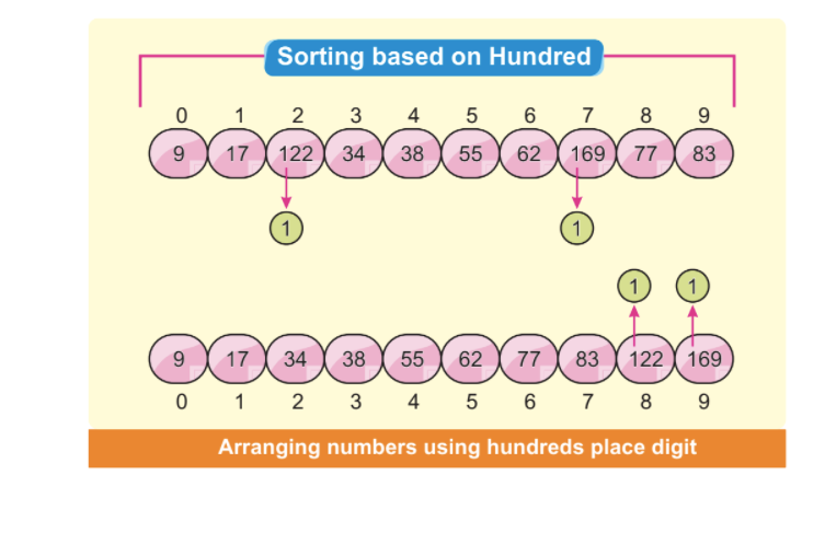
Our array is now fully sorted after arranging the elements based on the MSD.
We have understood the concepts of the Radix Sort Algorithm. But we need the Counting Sort Algorithm as one more algorithm to implement the Radix Sort. Now, let’s understand this counting sort algorithm.
A Counting Sort Algorithm
Here, we are going to explain each step of the counting sort algorithm:
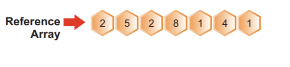
The previous reference array is our input array, and the numbers shown above the array are the index numbers of the corresponding elements.
Step 1: The first step in the counting sort algorithm is to search for the maximum element in the whole array. The best way to search for the maximum element is to traverse the whole array and compare the elements at each iteration; the greater value element is updated till the end of the array.
During the first step, we found the max element was 8 at the index position 3.
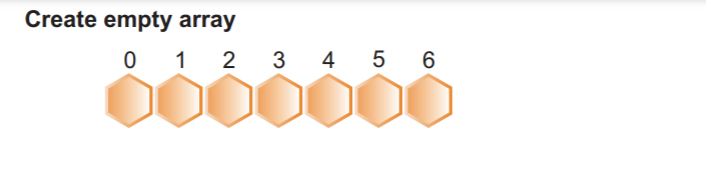
Step 2: We create a new array with the maximum number of elements plus one. As we already know, the maximum value of the array is 8, so there will be a total of 9 elements. As a result, we require a maximum array size of 8 + 1:
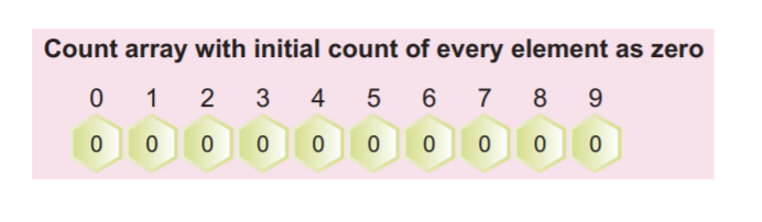
As we can see, in the previous image, we have a total array size of 9 with values of 0. In the next step, we will fill this count array with sorted elements.
Step 3: In this step, we count each element and, according to their frequency, fill in the corresponding values in the array:
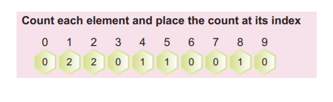
For example:
As we can see, element 1 is present two times in the reference input array. So we entered the frequency value of 2 at index 1.
Step 4: Now, we have to count the cumulative frequency of the filled array above. This cumulative frequency will be used later to sort the input array.
We can calculate the cumulative frequency by adding the current value to the previous index value, as shown in the following screenshot:
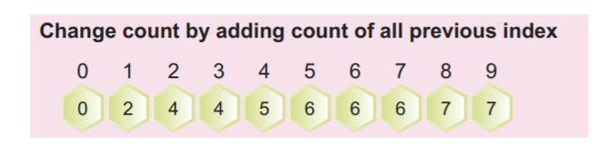
The last value of the array in the cumulative array must be the total number of elements.
Step 5: Now, we will use the cumulative frequency array to map each array element to produce a sorted array:
For example:
We choose the first element in array 2 and then the corresponding cumulative frequency value at index 2, which has a value of 4. We decremented the value by 1 and got 3. Next, we placed the value 2 in the index at the third position and also decremented the cumulative frequency at index 2 by 1.
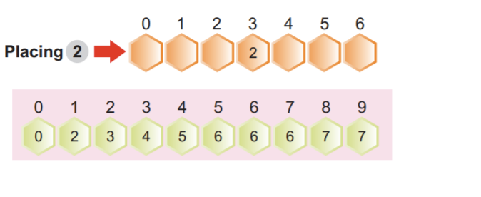
Note: The cumulative frequency at index 2 after being decremented by one.
The next element in the array is 5. We choose the index value of 5 in the commutative frequency array. We decremented the value at index 5 and got 5. Then, we placed array element 5 at index position 5. In the end, we decremented the frequency value at index 5 by 1, as shown in the following screenshot:
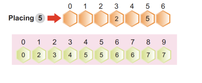
We do not have to remember to reduce the cumulative value at each iteration.
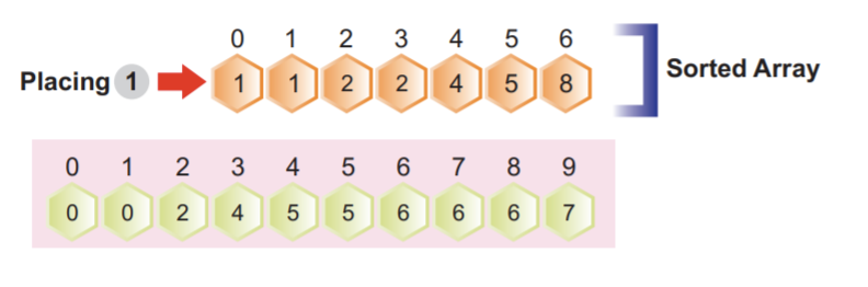
Step 6: We will run step 5 until every array element is filled in the sorted array.
After it is filled, our array will look like this:
The following C++ programme for the counting sort algorithm is based on the previously explained concepts:
using namespace std;
void countSortAlgo(intarr[], intsizeofarray)
{
intout[10];
intcount[10];
intmaxium=arr[0];
//First we are searching the largest element in the array
for (intI=1; imaxium)
maxium=arr[i];
}
//Now, we are creating a new array with initial values 0
for (inti=0; i<=maxium; ++i)
{
count[i] =0;
}
for (inti=0; i<sizeofarray; i++) {
count[arr[i]]++;
}
//cumulative count
for (inti=1; i=0; i--) {
out[count[arr[i]]–-1] =arr[i];
count[arr[i]]--;
}
for (inti=0; i<sizeofarray; i++) {
arr[i] = out[i];
}
}
//display function
void printdata(intarr[], intsizeofarray)
{
for (inti=0; i<sizeofarray; i++)
cout<<arr[i] <<“"\”";
cout<<endl;
}
intmain()
{
intn,k;
cout>n;
intdata[100];
cout<”"Enter data \”";
for(inti=0;i>data[i];
}
cout<”"Unsorted array data before process \n”";
printdata(data, n);
countSortAlgo(data, n);
cout<”"Sorted array after process\”";
printdata(data, n);
}
Output:
5
Enter data
18621
Unsorted array data before process
18621
Sorted array after process
11268
The following C++ programme is for the radix sort algorithm based on the previously explained concepts:
using namespace std;
// This function find the maximum element in the array
intMaxElement(intarr[], int n)
{
int maximum =arr[0];
for (inti=1; i maximum)
maximum =arr[i];
returnmaximum;
}
// Counting sort algorithm concepts
void countSortAlgo(intarr[], intsize_of_arr, int index)
{
constint maximum =10;
int output[size_of_arr];
int count[maximum];
for (inti=0; i< maximum; ++i)
count[i] =0;
for (inti=0; i<size_of_arr; i++)
count[(arr[i] / index) %10]++;
for (inti=1; i=0; i--)
{
output[count[(arr[i] / index) %10]–-1] =arr[i];
count[(arr[i] / index) %10]--;
}
for (inti=0; i0; index *=10)
countSortAlgo(arr, size_of_arr, index);
}
void printing(intarr[], intsize_of_arr)
{
inti;
for (i=0; i<size_of_arr; i++)
cout<<arr[i] <<“"\”";
cout<<endl;
}
intmain()
{
intn,k;
cout>n;
intdata[100];
cout<”"Enter data \”";
for(inti=0;i>data[i];
}
cout<”"Before sorting arr data \”";
printing(data, n);
radixsortalgo(data, n);
cout<”"After sorting arr data \”";
printing(data, n);
}
Output:
5
Enter data
111
23
4567
412
45
Before sorting arr data
11123456741245
After sorting arr data
23451114124567
Time Complexity of Radix Sort Algorithm
Let’s calculate the time complexity of the radix sort algorithm.
To calculate the maximum number of elements in the entire array, we traverse the entire array, so the total time required is O(n). Let’s assume the total digits in the maximum number is k, so total time will be taken to calculate the number of digits in a maximum number is O(k). The sorting steps (units, tens, and hundreds) work on the digits themselves, so they will take O(k) times, along with counting the sort algorithm at each iteration, O(k * n).
As a result, the total time complexity is O(k * n).
Conclusion
In this article, we studied the radix sort and counting algorithm. There are different kinds of sorting algorithms available on the market. The best algorithm also depends upon the requirements. Thus, it’s not easy to say which algorithm is best. But based on the time complexity, we are trying to figure out the best algorithm, and radix sort is one of the best algorithms for sorting. We hope you found this article helpful. Check the other Linux Hint articles for more tips and information.
from https://ift.tt/3GnoZQt


0 Comments