Pandas Tabulate

Pandas in Python can alter a Pandas DataFrame into a table with different styles. A Pandas DataFrame is executed using the “tabulate()” method. Let’s look at our examples and discuss the procedure to transform our Python DataFrame to the different styles of tables.

Syntax:
tabulate(DataFrame_object, headers=’keys’, tablefmt)

Parameters:

1. DataFrame_object refers to the existing DataFrame.
2. Headers keep the columns in the DataFrame after converting.
3. The tablefmt takes the table style.

We will see the different styles of tables by just modifying this parameter.

First, we create a DataFrame with 2 columns and we use this DataFrame in all table styles.

Note: Make sure to run this code in your environment because we use this code in all our examples. Otherwise, you will get errors.

import pandas
from tabulate import tabulate

# Consider the DataFrame having 5 records
dataset=pandas.DataFrame({
                        'Idea':['All','water supply','electricity','drilling','electricity'],
                        'demography':['ap','gujarat','patna','indore','norway']},index=[2,3,4,5,6])


print("Actual: \n")
print(dataset)

Output:

Actual:

           Idea demography
2           All         ap
3  water supply    gujarat
4   electricity      patna
5      drilling     indore
6   electricity     norway

Table 1: PSQL Format
Convert the DataFrame to psql format.

print(tabulate(dataset, headers='keys', tablefmt='psql'))

Output:

+----+--------------+--------------+
|    | Idea         | demography   |
|----+--------------+--------------|
|  2 | All          | ap           |
|  3 | water supply | gujarat      |
|  4 | electricity  | patna        |
|  5 | drilling     | indore       |
|  6 | electricity  | norway       |
+----+--------------+--------------+

Table 2: Fancy_Grid Format
Fancy_grid style is like organizing the DataFrame in a grid with neat margins.

print(tabulate(dataset, headers='keys', tablefmt='fancy_grid'))

Output:

╒════╤══════════════╤══════════════╕
│    │ Idea         │ demography   │
╞════╪══════════════╪══════════════╡
│  2 │ All          │ ap           │
├────┼──────────────┼──────────────┤
│  3 │ water supply │ gujarat      │
├────┼──────────────┼──────────────┤
│  4 │ electricity  │ patna        │
├────┼──────────────┼──────────────┤
│  5 │ drilling     │ indore       │
├────┼──────────────┼──────────────┤
│  6 │ electricity  │ norway       │
╘════╧══════════════╧══════════════╛

Table 3: Plain
Plain is similar to the plain DataFrame format. No margins are created in this format.

print(tabulate(dataset, headers='keys', tablefmt='plain'))

Output:

   Idea          demography
 2  All           ap
 3  water supply  gujarat
 4  electricity   patna
 5  drilling      indore
 6  electricity   norway

Table 4: HTML
The HTML code is returned as output when we specify the tablefmt as “html”. If you want to check whether the HTML code creates a table or not, run the generated HTML code in the browser.

print(tabulate(dataset, headers='keys', tablefmt='html'))

Output:

 <table>
<thead>
<tr><th style="text-align: right;">  </th><th>Idea        </th><th>demography  </th></tr>
</thead>
<tbody>
<tr><td style="text-align: right;"> 2</td><td>All         </td><td>ap          </td></tr>
<tr><td style="text-align: right;"> 3</td><td>water supply</td><td>gujarat     </td></tr>
<tr><td style="text-align: right;"> 4</td><td>electricity </td><td>patna       </td></tr>
<tr><td style="text-align: right;"> 5</td><td>drilling    </td><td>indore      </td></tr>
<tr><td style="text-align: right;"> 6</td><td>electricity </td><td>norway      </td></tr>
</tbody>
</table>

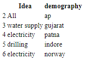
When you run this HTML code in the browser, you will see the following table:

Table 5: Github
Convert to “github” format.

print(tabulate(dataset, headers='keys', tablefmt='github'))

Output:

|    | Idea         | demography   |
|----|--------------|--------------|
|  2 | All          | ap           |
|  3 | water supply | gujarat      |
|  4 | electricity  | patna        |
|  5 | drilling     | indore       |
|  6 | electricity  | norway       |

Table 6: Pretty Format
The “pretty” format is same as the psql only.

print(tabulate(dataset, headers='keys', tablefmt='pretty'))

Output:

+---+--------------+------------+
|   |     Idea     | demography |
+---+--------------+------------+
| 2 |     All      |     ap     |
| 3 | water supply |  gujarat   |
| 4 | electricity  |   patna    |
| 5 |   drilling   |   indore   |
| 6 | electricity  |   norway   |
+---+--------------+------------+

Table 7: TCSV Format
If you want to see your DataFrame in the tab which is separated by CSV, you can use “tcsv”.

print(tabulate(dataset, headers='keys', tablefmt='tsv'))

Output:

     Idea           demography
 2  All             ap
 3  water supply    gujarat
 4  electricity     patna
 5  drilling        indore
 6  electricity     norway

Table 8: CSV Format
Convert the DataFrame to csv format.

print(tabulate(dataset, headers='keys', tablefmt='csv'))

Output:

    Idea          demography
--  ------------  ------------
 2  All           ap
 3  water supply  gujarat
 4  electricity   patna
 5  drilling      indore
 6  electricity   norwayApplied necessary capitalization since this is a subheading.

Table 9: Excel format
Convert the DataFrame to excel format. This is similar to CSV.

print(tabulate(dataset, headers='keys', tablefmt='excel'))

Output:

    Idea          demography
--  ------------  ------------
 2  All           ap
 3  water supply  gujarat
 4  electricity   patna
 5  drilling      indore
 6  electricity   norway

Conclusion

When rendering a DataFrame into a table code, we first need to import the tabulate module. We just change the tablefmt parameter to set the table style. By seeing the 8 styles, we came to know that Pandas have such a wonderful option to display the DataFrame in different ways that meet our project requirements. Make sure that you set the headers parameter to “keys”.

from https://ift.tt/f5xUil6