Ensemble Learning in Python by Example

There is no secret that machine learning is getting better with time and the predictive models. Predictive models form the core of machine learning. It is good to improve the accuracy of the model for better results in the machine learning model. A technique called “ensemble machine learning” is used for increasing the performance and accuracy of a model.

Ensemble learning uses different models of machine learning for trying to make better predictions on the dataset. A model’s predictions are combined in an ensemble model for making the final prediction successful. However, many people are not familiar with ensemble machine learning. Read below; we explain everything about this machine learning technique using Python with appropriate examples.

Suppose you are participating in a trivia game and have good knowledge of some topics, but you don’t know anything other few topics. A team member would be required to cover all of the game topics if you wish to achieve a maximum score in the game. It is the basic idea behind ensemble learning in which we combine the predictions from different models for accurate output.

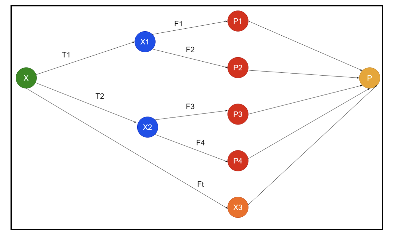
The picture shows an example of schematics of an ensemble. In the above image, the input array is filled by three preprocessing pipelines, and there are base learners. All ensembles combine the predictions of the base learners into the final prediction array “P”.

Suppose you are thinking about combining all of the predictions. If we consider the above example, it is easy to answer when you have a team; machine learning is the same as the classification problems. In machine learning, the system takes a most common class label prediction equivalent to the majority rule. However, there are different ways to combine various predictions, and you can use a model for learning to combine the predictions appropriately.

What is Ensemble Learning?

Machine learning and statistics are spreading worldwide, so we need different techniques to increase a predictive model’s performance for better accuracy. Ensemble learning is a procedure for using different machine learning models and constructing strategies for solving a specific problem.

The ensemble combines different sets of models for improvising on predictive power and stability. According to the Ensemble-based models, there are two different scenarios, i.e., a higher or lower amount of data.

Let’s understand the ensemble learning using an example; suppose we want to invest in the “ABC” company, but we are not sure about its performance. So we take advice from different people about the performance of the “ABC” company. We may take the advice from:

Employees of “ABC” company: Employees of the company know everything about the company’s internal functionality and all of the inside information. However, employees lack a wider perspective about the competition, how the technology is evolving, and the effects on the “ABC” company’s product. According to the information and past experiences, having advice from employees is 65% times right.

Financial Advisors of “ABC” company: Financial advisors have a wider perspective about the competitive environment. However, the advice from the financial advisor of the company has been 75% times correct in the past.

Stock Market Traders: These traders always observe the company’s stock price, and they know the seasonal trends and overall market performance. They also develop a keen institution about the variation of stocks over time. Still, the advice of stock market traders has been 70% times helpful in the past.

Employees of the Competitor’s Company: These employees know the internal functionalities of a competitor’s company and are aware of the specific changes. However, they don’t have every sight of their company and external factors related to the competitor’s growth. Still, employees of the competitor’s company were 60% times right in the past.

Market Research Team: This team works to analyze the customer preferences of “ABC” company’s product over the competitors. This team deals with the customer side to be unaware of the variation “ABC” company will bring due to the alignment to their goals. However, the market research team was 75% times helpful in the past.

Social Media Expert Team: This team is beneficial to understand how “ABC” company’s products are positioned in the market. They also analyze the customer’s sentiments changing with the company over time. Social media expert team unaware of any information beyond digital marketing. So, they are 65% times right in the past.

In the above scenario, we have different aspects of making a good decision as the accuracy rate can be 99%. However, the assumptions we have used above are independent and slightly extreme because they are expected to be correlated.

Ensemble Methods

Now let’s discuss the complete information of the different techniques of ensemble learning in Python:

Basic Ensemble Method

There are three types of techniques in the basic ensemble method, and they are:

Max Voting

The major work of max voting is used to solve classification problems. This method has multiple independent models, and the individual output is known as “vote”. Multiple models are used for predicting every data point. The class with a maximum vote will return as an output. The prediction that users get by the majority of the model will be used as a final prediction.

For example, we have five experts for rating a product, they have provided the ratings like this:

Expert 1	Expert 2	Expert 3	Expert 4	Expert 5	Final Rating
4	5	4	5	4	4

Here is the sample code for the above example:

model1 = tree.DecisionTreeClassifier()

model2 = KNeighborsClassifier()

model3= LogisticRegression()

model1.fit(x_train,y_train)

model2.fit(x_train,y_train)

model3.fit(x_train,y_train)

pred1=model1.predict(x_test)

pred2=model2.predict(x_test)

pred3=model3.predict(x_test)

final_pred = np.array([])

for i in range(0,len(x_test)):

final_pred = np.append(final_pred, mode([pred1[i], pred2[i], pred3[i]]))

In the above sample code, x_train is an independent variable of the training data, and y_train is a target variable of the training data. Here x_train, x_test and y_test are validation sets.

Averaging

There are multiple predictions made for every data point in the averaging; it is used for the regression problem. In this technique, we find an average of multiple predictions from the given models then uses this average to obtain a final prediction.

The averaging method has independent models which are used to find the average of the predictions. Generally, the combined output is more accurate than the individual output as the variance is decreased. This method is used to make appropriate predictions in the regression problem or find the possibility of the classification problem.

If we consider the above example, then the average of the ratings will be

Expert 1	Expert 2	Expert 3	Expert 4	Expert 5	Final Rating
4	5	4	5	4	4

average of the ratings = (4+5+4+5+4+4)/5 = 4.4

Sample code for the above problem will be:

model1 = tree.DecisionTreeClassifier()

model2 = KNeighborsClassifier()

model3= LogisticRegression()

model1.fit(x_train,y_train)

model2.fit(x_train,y_train)

model3.fit(x_train,y_train)

pred1=model1.predict_proba(x_test)

pred2=model2.predict_proba(x_test)

pred3=model3.predict_proba(x_test)

finalpred=(pred1+pred2+pred3)/3

Weighted Average

This method is an extended type of the average method as models are assigned various weights that define the importance of every model for proper prediction. For example, if a team has two experts and two beginners, the importance will be given to the experts instead of the beginners.

The result of the weighted average can be calculated as [(5×0.24) + (4×0.24) + (5×0.19) + (4×0.19) + (4×0.19)] = 4.68.

Factors	Expert 1	Expert 2	Expert 3	Expert 4	Expert 5	Final rating
weight	0.24	0.24	0.19	0.19	0.19
rating	5	4	5	4	4	4.68

Sample code for the above example of weighted average:

model1 = tree.DecisionTreeClassifier()

model2 = KNeighborsClassifier()

model3= LogisticRegression()

model1.fit(x_train,y_train)

model2.fit(x_train,y_train)

model3.fit(x_train,y_train)

pred1=model1.predict_proba(x_test)

pred2=model2.predict_proba(x_test)

pred3=model3.predict_proba(x_test)

finalpred=(pred1*0.3+pred2*0.3+pred3*0.4)

Advanced Ensemble Methods

Stacking

Stacking method, multiple models such as regression or classification are combined through a meta-model. In other words, this method uses different predictions from various models for building a new model. All of the base models are properly trained on the dataset, and then a meta-model is properly trained on features returned from base models. Hence, a base model in stacking is specifically different, and the meta-model is beneficial for finding the features from the base model to obtain great accuracy. Stacking has a specific algorithm step as below:

• First, train a dataset in n parts.
• The base model will be fitted in the n-1 parts, and predictions are divided in the nth part. It requires to be performed for every nth part of a train set.
• The model will be fitted on a complete train dataset, and this model will be used to predict a test dataset.
• After that, the prediction on a train data set will be used as a feature to create a new model.
• At last, the final model will be used for predicting on a test dataset.

Blending

Blending is the same as the stacking method, but it uses a holdout set from a train set for making the predictions. In simple words, blending uses a validation dataset and keeps it separated for making the predictions instead of using a complete dataset to train a base model. So here are the algorithmic steps we can use in the blending:

• First, we need to split training datasets into different datasets such as test, validation, and training dataset.
• Now, fit the base model by a training dataset.
• After that, predict the test and validation dataset.
• The above predictions are used as a feature for building the second-level model.
• Finally, the second level model is used for making the predictions on the test and meta-feature.

Bagging

Bagging is also called a bootstrapping method; it combines results of different models for obtaining generalized results. In this method, a base model runs on the bags or subsets to obtain a fair distribution of a complete dataset. These bags are subsets of a dataset with the replacement for making the size of a bag similar to a complete dataset. The output of bagging is formed once all of the base models are combined for the output. There is a specific algorithm for begging as below:

• First, create different datasets from a training dataset by choosing observations with a replacement.
• Now, run base models on every created dataset independently.
• Finally, combine all of the predictions of the base model with every final result.

Boosting

Boosting works to prevent the wrong base model from impacting a final output, rather than combining a base model, boosting focused on creating a new model dependent on a previous one. This new model removes all previous models’ errors, and every model is known as a weak learner. The final model is called a strong learner, created by getting a weighted mean of the weak learners. It is a sequential procedure in which every subsequent model works to correct errors of previous models. Following are the sequential steps of the algorithm for boosting:

• First, take the subset of a training dataset and then train the base model on the dataset.
• Now, use the third model for making predictions on a complete dataset.
• After that, calculate the error by the predicted and actual value.
• Once calculate the error, then initialize the data point with the same weight.
• Now, assign a higher weight to the incorrectly predicted data point.
• After that, make a new model by removing the previous errors and make appropriate predictions by the new model.
• We need to create different models–each successive model by correcting the errors of the last models.
• Finally, the strong learner or final model is a weighted mean of the previous or weak learner.

Conclusion

That concludes our detailed explanation of ensemble learning with the appropriate examples in Python. As we have mentioned earlier, ensemble learning has multiple predictions, so in other words, we use multiple models to find the most accurate output possible. We have mentioned types of ensemble learning with examples and algorithms of them. There are multiple methods to find out the results using multiple predictions. According to many data scientists, ensemble learning offers the most accurate output possible as it uses multiple predictions or models.

from Linux Hint https://ift.tt/2RgqySn